Principal Component Analysis (PCA) demonstration

This demo presents the PCA as an algorithm useful for feature reduction and final data classification. The goal consists on computing principal components for a data set composed by 100 heartbeats coming from a real electrocardiographic record (ECG). In this way we want to improve the dataset presentation for the final data classification. Heartbeats have been previously selected in order to include two different classes (44 objects fro the class 1 and 56 from the class 2). In addition, we have downsampled them to 25 samples for beat in order to drastically reduce the size of the dataset.

Load data
Dataset presentation
Principal Component Analysis
Selecting the features
Reducing the features

Load data

The variable ecg is sized 100 by 25 so that means 100 heartbeats (observations) sampled at 25 segments (features) each.

load ecg;
figure('Name','ECG dataset', 'NumberTitle','off');
plot(ecg(1,:),'o:r', 'LineWidth',2);
hold; plot(ecg(100,:),'o:b', 'LineWidth',2);
title('The two classes for the ECG dataset')
xlabel('samples');
ylabel('amplitude (mV)');
nobservations=size(ecg,1)
nfeatures=size(ecg,2)

Current plot held

nobservations =

   100


nfeatures =

    25

Dataset presentation

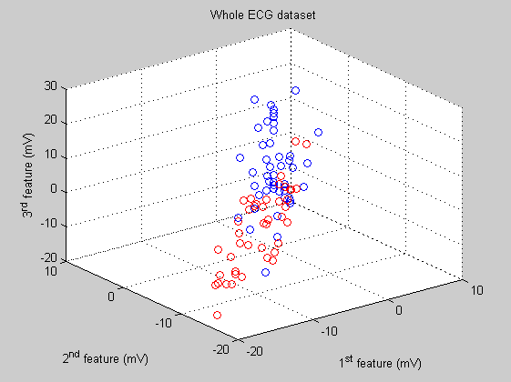
If we show the whole dataset (3D scatter plot) selecting three of the 25 features that compose each observation we can not distinguish the two classes. Both classes appear mixed togheter.

feature_1=1;
feature_2=2;
feature_3=3;
figure('Name','ECG dataset', 'NumberTitle','off');
scatter3(ecg(:,feature_1),ecg(:,feature_2),ecg(:,feature_3),[],labels);
title('Whole ECG dataset')
xlabel('1^{st} feature (mV)');
ylabel('2^{nd} feature (mV)');
zlabel('3^{rd} feature (mV)');

Principal Component Analysis

Now we use PCA in order to compute the coefficients the principal components coeff and the component's values score in the new orthogonal space. The variable latent contents the eigenvalues of the covariance matrix of ingredients. To perform principal components analysis with standardized variables, that is, based on correlations, we use princomp(zscore(ecg)).

[coeff,score,latent,tsquare] = princomp(zscore(ecg));

Selecting the features

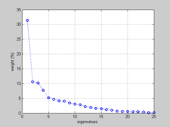
in this stage we are going to slect those features that include the maximum data variance as possible. In this case we present percentually the eigenvalues in a 2D plot. Resulting from the plot, the 1st, 2nd and 3rd features include more that the 50% of the data variance.

percent=latent./sum(latent)*100;
figure('Name','PCA eigenvalues', 'NumberTitle','off');
plot(1:length(latent),percent,'o:b', 'LineWidth',2);
grid;
xlabel('eigenvalues');
ylabel('weight (%)');

Reducing the features

Now we reduce the data features' to the 1st, 2nd and 3rd principal components. Consequently the classification of the heartbeats in the set is clearly improved.

figure('Name','3D Reduced PC', 'NumberTitle','off');
scatter3(score(:,1),score(:,2),score(:,3),[],labels);
title('Reduced set by PCA');
xlabel('1^{st} feature (mV)');
ylabel('2^{nd} feature (mV)');
zlabel('3^{rd} feature (mV)');

figure('Name','PC reduced vs NOT reduced dataset', 'NumberTitle','off');
subplot(1,2,1); scatter(score(:,1),score(:,2),[],labels);
title('Reduced set');
xlabel('1^{st} feature (mV)'); ylabel('2^{nd} feature (mV)');
subplot(1,2,2); scatter(ecg(:,feature_1),ecg(:,feature_2),[],labels);
title('NOT reduced set');
xlabel('1^{st} feature (mV)'); ylabel('2^{nd} feature (mV)');