6th week CMR data classification and analysis

Starting from the data generated by the 6th week Cardiovascular Magnetic Resonance (CMR) tests (2794 observations sized 18 features each) we perform a Principal Component Analyis (PCA) in order to reduce dimensionality and best interpret the data.

Load and present original data
Principal Complonent Analysis
PCA 2D Plots
PCA 3D Plots
Clustering

Load and present original data

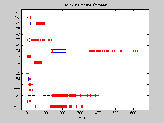
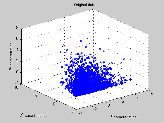
In this case the original matrix has been composed by means of the 2704 CMR experiments featured by 18 measurements each. Consequently the matrix is sized 2704 by 18. A boxplot is presented too. Measured features are defined in the features variable. On the other hand and in order to get the 2D and 3D plots, we select from the original data the three most sparse variables, let's say, P4, P21 and P11 (as you can check in the boxplot).

load Data6thWeek;
figure('Name','-----> Boxplot for the original 6th WEEK data plots', 'NumberTitle','off');
boxplot(data, 'orientation','horizontal', 'labels',features'); title('CMR data for the 1^{st} week');

[sorted,indexes]=sort(std(data));
ind1=indexes(end);
ind2=indexes(end-1);
ind3=indexes(end-2);
features{ind1}, features{ind2}, features{ind3}

ans =

P4


ans =

E21


ans =

E11

Principal Complonent Analysis

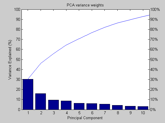
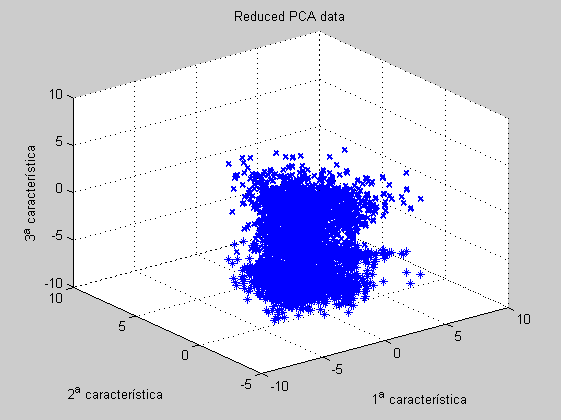
First at all we center and scale the data matrix. Next, we reduce the number of variables by means of the PCA algorithm. The selected variables are all those that best explain the data dispersion. In this case, the variance included with the 6th, 2nd and 3rd PC is about the 54%.

dataz=zscore(data);
[coefs,scores,variances,t2]=princomp(dataz);

percent_explained=100*variances/sum(variances);
figure('Name','-----> PARETO chart for the 6th WEEK data plots', 'NumberTitle','off');
pareto(percent_explained); title('PCA variance weights'); xlabel('Principal Component'); ylabel('Variance Explained (%)');

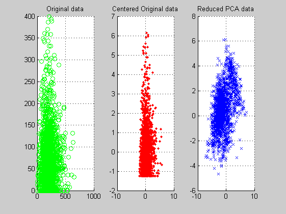
PCA 2D Plots

From the 2D PCA reduced features data plots we get the intuition that the data appear oriented into a double lobe structure. Maybe a later clustering processing reveals differences between the two lobes.

figure('Name','-----> 2 feature 6th WEEK data plots', 'NumberTitle','off');
subplot(1,3,1); scatter(data(:,ind1),data(:,ind2),'og'); title('Original data'); grid;
subplot(1,3,2); scatter(dataz(:,ind1),dataz(:,ind2),'.r'); title('Centered Original data'); grid;
subplot(1,3,3); scatter(scores(:,1),scores(:,2),'xb'); title('Reduced PCA data'); grid;

PCA 3D Plots

From the 3D PCA reduced features we confirm the 2-lobe structure commented above.

figure('Name','-----> 3 features 6th WEEK data plots', 'NumberTitle','off');
scatter3D(dataz(:,ind1),dataz(:,ind2),dataz(:,ind3)); title('Original data');
figure('Name','-----> 3 features 6th WEEK data plots', 'NumberTitle','off');
scatter3D(scores(:,1),scores(:,2),scores(:,3)); title('Reduced PCA data');
figure('Name','-----> 3 features 6th WEEK data plots: BIPLOT tool', 'NumberTitle','off');
biplot(coefs(:,1:3),'scores',scores(:,1:3), 'varlabels',features);

Current plot held
Current plot held

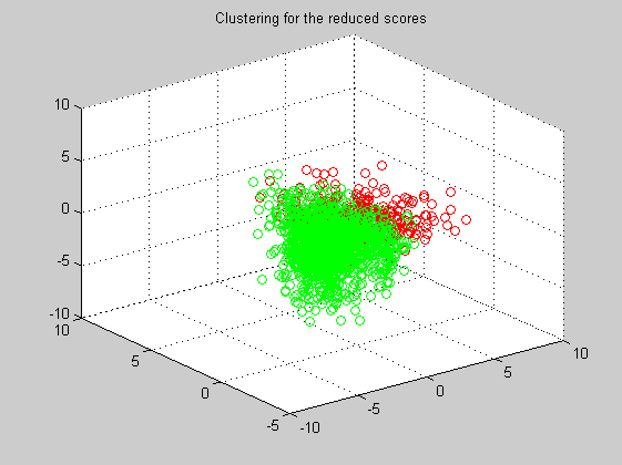
Clustering

Now, and using the PCA information, we apply the MaxMin clustering algorithm. At the first iteration we manually select the two centroids that will be the origin of the two clusters.

dist=pdist(scores(:,1:3),'euclidean');
sq_dist=squareform(dist);
centroids=[1783 1411];
labels=maxmin('min',sq_dist,centroids);
for i=1:length(labels)
    if (labels(i) == 1) marker(i,:)=[1 0 0];
    else marker(i,:)=[0 1 0];
    end
end
figure('Name','-----> Clustering 6th iteration', 'NumberTitle','off');
scatter3(scores(:,1),scores(:,2),scores(:,3),[],marker);
title('Clustering for the reduced scores');